A pivot table enables you to calculate, summarize, and analyze data for comparisons, patterns, and trends. A video about pivot tables in this course reviews the steps to create a pivot table. You can replay the video, if needed.
Another reading in this course that covers sorting and filtering in spreadsheets offers two examples of how sorting and filtering enables certain insights. This reading uses the same examples from the sorting and filtering reading. The examples are repeated to show how pivot tables enable the same insights more quickly.
Description of spreadsheet
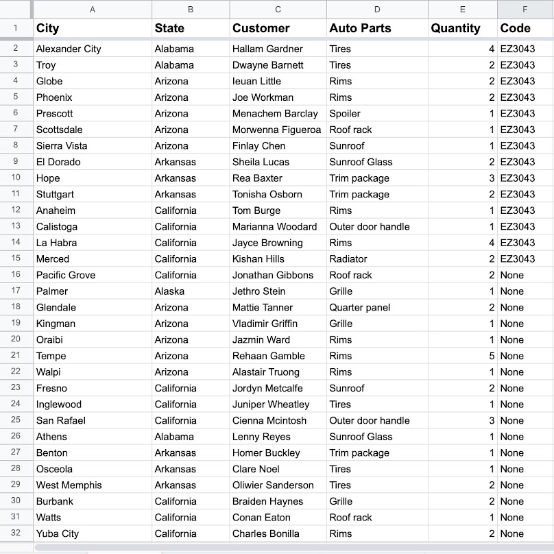
Suppose you have a spreadsheet that contains online sales data, like the one shown in the image below. Recall from the video that a cell in a spreadsheet holds the data. Columns are vertical and are labeled alphabetically. Rows are horizontal and are labeled numerically. People refer to cell positions by combining the column and row designation, like cell A2. In the sample online sales data below, cell A2 contains the data, Alexander City.
Spreadsheet contains city, state, customer, auto parts, quantity, and code data in Columns A through F.
A pivot table in this spreadsheet enables you to gather insights like these:
- Number and percentage of purchases made from each campaign (by campaign codes)
- Campaign-related purchases (overall and by state)
Example 1: Purchases made from each campaign
With sorting and filtering, you determine the number of purchases per campaign code by filtering for one code at a time. With a pivot table, you can view the number of purchases per campaign code all at once. This can save you time when working with a large amount of data.
1. Create the pivot table with Code as the Columns and State as the Rows, and then add Code as a Value summarized by COUNTA.
In the pivot table editor, State under Rows and Code under Columns are sorted in ascending order with Show totals checked. In the pivot table editor, State under Rows and Code under Columns are sorted in ascending order with Show totals checked. Code under Value is summarized by COUNTA.

The resulting pivot table is similar to the one shown below, where the number of purchases for each campaign is shown in the row labeled Grand Total.
Note: Some rows (states) in the pivot table have been hidden to save space and show the counts at the bottom of the table.
A pivot table. Counts for each code for each state; grand totals for codes in columns and grand totals for states in rows.

2. You can then insert a formula to calculate the percentage of total purchases by dividing each grand total by 569. The formula in cell D54 is: =D53/569 which takes the value in cell D53, or 28, and divides it by 569. The resulting percentage is 4.92% for Campaign 39343E. Copy this formula to cells E54 and F54 to calculate the percentages for the other two campaigns.
Using the the pivot table and subsequent calculations, you could share the following information with stakeholders:
- 4.92% of all purchases resulted from Campaign 39343E
- 2.81% of all purchases resulted from Campaign CGRWAT
- 2.64% of all purchases resulted from Campaign EZ3043
Conclusion
The pivot table returned the same results as sorting and filtering the Code column and manually counting instances for each code.
Instead of filtering for each state one at a time to get the counts per code, each state’s count is already summarized in Column G (grand total) in the pivot table. But now you need a count of the non-campaign related purchases. If you insert None in the data as the campaign code for non-campaign purchases, the pivot table automatically adds another count for None in Column G.
An additional column was added for “None” to count the purchases made without a code to include them in grand total.

Finally, you can insert a formula in Column I to calculate the percentage of campaign-related purchases for each state. In cell I4, enter =(D4+E4+F4)/H4. Next, copy and paste the contents of cell I4 into all remaining cells in Column I.
A pivot table. Column to the right of Grand Total calculates the percentage of campaign-related purchases for each state.

For example, after copying and pasting the contents from cell I4 to cell I6, the formula in cell I6 for Arizona becomes =(D6+E6+F6)/H6 which adds the values from the three campaigns and divides that sum by the grand total of purchases in Arizona.
Calculation in cell I6: =(1+1+5)/25 = 0.28, or 28%
Using the calculations for campaign-related purchases, you could share the following information with stakeholders:
- 22% of purchases in Alabama were campaign-related
- 0% of purchases in Alaska were campaign-related
- 28% of purchases in Arizona were campaign-related
- (and so on for each subsequent state in the U.S.)
Conclusion
The pivot table returned the same results as filtering the State column state by state to get a breakdown of the data by state. However, using the pivot table saved some time!
Resources for more information
You can refer to the following resources for more information about working with pivot tables:
- Create and edit pivot tables: Instructions to create pivot tables in Google Sheets
- Create a PivotTable to analyze worksheet data: Help creating pivot tables in Microsoft Excel